The goal of this document is provide some basic performance testing of the optmatch package. In most matching workflows, a user first creates distances, produces one or more matches, assesses balance on a given match, and, provided balance meets necessary requirements, proceeds to analysis. Of these tasks, optmach is responsible for distance creation and creating the match. These two tasks will be considered separately. The remainder of this document lays out the performance testing strategy and then implements it for the distance creation and matching routines in optmatch.
Performance Testing Strategy
R provides built in execution profiling through the Rprof function (and a similarly named command line option). When invoked, this function regularly interrupts normal processing and writes out the current call stack to a file. This information can be used to attribute the portion of run time attributable different functions.
For interpretation of this data, we rely on the profr package, which provides some graphical summaries to help make raw profile data more manageable.
Since we suspect that creation of large data sets may account for a sizeable portion of the runtime of large problems, we also profile memory usage with simulated data described in its own section.
Simulated Data
Before proceeding to the actual profiling, we begin by creating some simulated data.1 We use 1000 individuals, with 442 receiving the treatment condition. Treatment assignment is based on a simple linear model of 3 covariates (two Normal variables and one categorical variable with 5 levels).
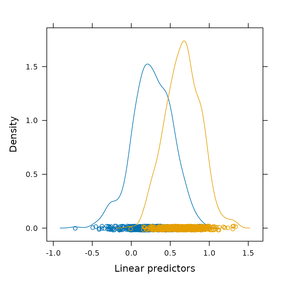
For most of the problems, we create a model of treatment assignment and then pull out the linear predictors from that model. Figure 1 shows the distributions of the predicted probabilities for the treated and control groups (henceforth the propensity score).

Figure 1. Relative distribution of predicted probabilities for simulated treated and control units.
Distance Creation
We begin by benchmarking dense distance creation.2 The match_on.numeric method has the least complicated interface and applies the least pre-processing to the input. Figure 2 shows the profile data for using match_on.numeric with the propensity score.
Figure 2. Profiling diagram for dense distance creation for
N = r N units.
There are two ways to create sparse problems. In the first, we use the caliper argument (for the numeric and glm methods of match_on). This argument looks over all the treated and control values and computes which treated and control units should be compared, and then computes the exact distances between them. Applying a caliper width of 1 to the simulated data, leads to a sparse matrix with 23.7% finite entries. Figure 3 shows the profiling data for this process.
The alternative to the caliper argument is the within argument. This method is more general, applying to all match_on methods, but can sometimes require generating a dense matrix first (though not always — the exactMatch function doesn’t require a dense matrix). To use the within argument, we use exactMatch create two subproblems based on the categorical covariate. 12.9% finite entries. Figure 4 shows the profiling results when using the within argument.
Figure 3. Profiling diagram for caliper based sparse distance creation
for N = r N units.
Figure 4. Profiling diagram for within based sparse distance creation
for N = r N units.
match_on Methods
These additional methods add some pre-processing to the distance creation. These methods can work on sparse problems, but to keep things simple, these examples just create dense matrices. The glm method is a relatively small wrapper around the numeric method used in the previous examples. Figure 5 shows the profiling data for glm method, which we would expect to look very similar to Figure 2, the dense matrix problem from the previous section.
Figure 5. Profiling diagram for glm distance creation
for N = r N units.
Figure 6 shows the profiling data for using the formula method. This method, by default, creates a squared Mahalanobis distance between treated and control pairs (Euclidean distances scaled by the variance-covariance matrix). Figure 6 shows the profiling data for using the formula method. This plot is expected to be very different than the previous as all the previous examples were based a simple absolute difference of a 1-D vector. In this task, however, we have to compute a variance-covariance matrix and then produce a series of multiplications to compute the squared distances. There may be opportunities to improve both components of the distance creation. Additionally, they may not scale in the same way, with one dominating for small problems and the other for large. This plot does not provide any information the scaling nature of the function.
Figure 6. Profiling diagram for formula (Mahalanobis) distance creation
for N = r N units.
Matching
Now that distance creation code has been benchmarked, we now consider the matching process itself. We reuse the earlier distance objects. To keep things simple, most of these matches will be computed using fullmatch at default settings. The process of matching, as currently implemented in optmatch can be broken down into the following steps:
We should expect to see these phases in each of the next figures. Figure 7 shows the matching process applied to the dense distance matrix from the previous section. Figure 8 shows a profiling information for the caliper argument based sparse distance matrix. Figure 9 shows the profiling data for the stratified, sparse problem (which can be split up into separate calls to the solver)
#> Warning in fullmatch(result.dense): Without 'data' argument the order of the match is not guaranteed
#>     to be the same as your original data.
Figure 7. Profiling diagram for dense matrix based matching for
N = r N units.
#> Warning in fullmatch(result.sparse.caliper): Without 'data' argument the order of the match is not guaranteed
#>     to be the same as your original data.
Figure 8. Profiling diagram for sparse matrix based matching for
N = r N units.
#> Warning in fullmatch(result.sparse.within): Without 'data' argument the order of the match is not guaranteed
#>     to be the same as your original data.
Figure 9. Profiling diagram for stratified sparse matrix based matching
for N = r N units.
The previous tests used fullmatch with the default arguments. To test out the use of the various constraint arguments, we call pairmatch on the dense distance problem. In addition to fixing the minimum and maximum number of controls per matched set to 1, the pairmatch function inspects the distance object to set appropriate values for omit.fraction, the argument that allows a portion of the control group to be discarded. Figure 10 shows these profiling data.
#> Warning in fullmatch(x = x, min.controls = controls, max.controls = controls, : Without 'data' argument the order of the match is not guaranteed
#>     to be the same as your original data.
Figure 10. Profiling diagram for dense matrix pairmatching for
N = r N units.
mdist and match_on
In version 0.7 of optmatch and earlier, the primary method of creating distances was to use the mdist function. In version 0.8, match_on was added as a more comprehensive tool, specifically one that allowed for arbitrary sparseness of distances matrices.
#> Intervals smaller than ~5ms will probably not result in accurate timings.
#> Warning in Rprof(prof_output, interval = 0.001, line.profiling = TRUE,
#> gc.profiling = TRUE, : interval too short for this platform, using '0.010000'
#> Warning in mdist(model, structure.fmla = ~X3): 'mdist' is deprecated.
#> Use 'match_on' instead.
#> See help("Deprecated")
Figure 11. Profiling results for a stratified mdist distance problem.
Appendix
Scaling
#> Warning in mdist(z ~ data): 'mdist' is deprecated.
#> Use 'match_on' instead.
#> See help("Deprecated")
#> Warning in mdist(z ~ data): 'mdist' is deprecated.
#> Use 'match_on' instead.
#> See help("Deprecated")
#> Warning in mdist(z ~ data): 'mdist' is deprecated.
#> Use 'match_on' instead.
#> See help("Deprecated")
#> Warning in mdist(z ~ data): 'mdist' is deprecated.
#> Use 'match_on' instead.
#> See help("Deprecated")
#> Warning in mdist(z ~ data): 'mdist' is deprecated.
#> Use 'match_on' instead.
#> See help("Deprecated")
#> Warning in mdist(z ~ data): 'mdist' is deprecated.
#> Use 'match_on' instead.
#> See help("Deprecated")
#> Warning in mdist(z ~ data): 'mdist' is deprecated.
#> Use 'match_on' instead.
#> See help("Deprecated")
#> Warning in mdist(z ~ data): 'mdist' is deprecated.
#> Use 'match_on' instead.
#> See help("Deprecated")
#> Warning in mdist(z ~ data): 'mdist' is deprecated.
#> Use 'match_on' instead.
#> See help("Deprecated")
#> Warning in mdist(z ~ data): 'mdist' is deprecated.
#> Use 'match_on' instead.
#> See help("Deprecated")
#> Warning in mdist(z ~ data): 'mdist' is deprecated.
#> Use 'match_on' instead.
#> See help("Deprecated")
#> Warning in mdist(z ~ data): 'mdist' is deprecated.
#> Use 'match_on' instead.
#> See help("Deprecated")
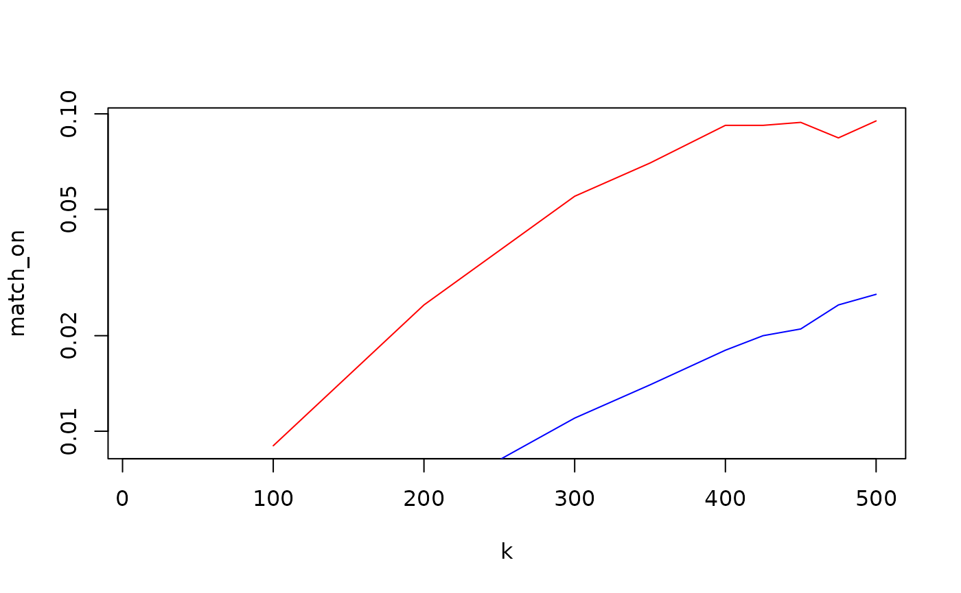
This section considers how the two functions scale up as the problem
size gets bigger. We create problems sets of size N = 2K
with K treatment and K control units. Figure
12 shows the run time of the two functions as K is
increased. The y axis is logged showing that both methods
grow roughly quadratically, as we would expect from the nature of the
algorithms. Of course, the absolute run time of
match_on is orders of magnitude worse.
#> Warning in xy.coords(x, y, xlabel, ylabel, log): 1 y value <= 0 omitted from
#> logarithmic plot
Figure 12. Run times for increasingly large problems for the match_on (red) and mdist (blue) functions.